Sunday 27 June 2010

Rotating Source

When considering a rotating observer, the change in velocity will be a reciprocal component generated from rotary motion and will vary the frequency, dependent on the source distance, revolutions per minute (rpm) and angular position.

(picture from http://www.daerospace.com/MechanicalSystems/DwellLinkFig1.png)


The system has a relationship similar to that of the crank and shaft mechanism pictured above and a mathematical representation similar to piston equations, describing rotary motion converted into reciprocal.

  • L = length of rod (distance between piston join and crank join)
  • r = crank radius
  • theta = angular velocity
  • x = reciprocal displacement
Angular velocity


to get the velocity with respect to angular position, we differentiate using chain rule:


to get the velocity with respect to time:


Plotting the relationship between angular position and change in reciprocating velocity, we find that when the source is far away, the relationship represents one that is sinusoidal in nature and as it gets closer, it converges on a tangential relationship.


Graph above is the reciprocating velocity relationship, head size 20cm and source distance 30cm.

Graph above is the reciprocating velocity relationship, head size 20cm and source distance 1 metre.


Rotating Binaural Dummy Head


Using the change in velocity from the above graph and putting it into the equation for doppler effect as a variable, the relationship for change in frequency can be found.


In the graph above, the line that is positive from 0 to (pi) and then negative between (pi) and 2(pi) is the left ear of the binaural microphones. The above equation in the graph describes this relationship. The other line on the graph corresponds to the lower equation and is the same as the upper equation, with a half-phase difference.

The change in frequency can be seen on the y-axis, only varying 6 Hz, changing from 503 - 497Hz and having a rest frequency of 500Hz.


Above image shows the effect of the rotating binaural dummy head at 500Hz.
Rotating at 84.5rpm

Thursday 17 June 2010

Doppler Effect

Doppler effect describes the frequency of a moving source past an observer, for example a siren on an emergency vehicle speeding past a stationary observer.


"Doppler effect from ambulance siren binaurally"

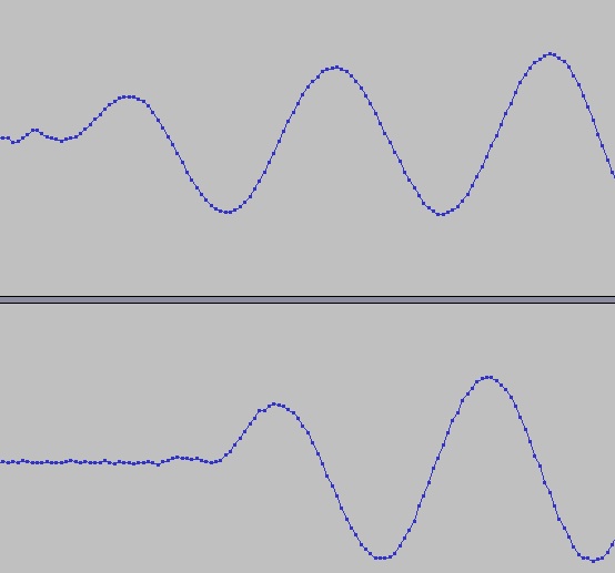
Ambulance Doppler Effect recorded using binaural microphones

(recorded in the meadows, edinburgh 17/06/2010)

From measuring the change in the ambulances pitch, you could effectively calculate the velocity that it is traveling. This is how speed guns work and how we are able to calculate the relative speed of distant astronomical objects using the Doppler effect.

The effect on the frequency that the observer hears, is one that begins high and gradually decreases before becoming the frequency that it produces at rest, directly in front of the observer. This is due to the sound being compressed by the vehicles motion, relative to the observer.

When the vehicle has passed and is moving away from the observer, the frequency decreases again, as the sound waves produced on the vehicle are being stretched by the vehicles motion, relate to the observer.

The same effect also happens for light relative to a stationary observer, positioned at (p4) in the diagram below (showing how light is shifted for a traveling observer). The below diagram shows that, for a stationary observer at position (p4) with sound travelling from left to right, the waves are compressed as they approach the observer and as they pass and travel away from the observer, they are expanded. Also, notice how the expansion and compression will be different for a source that passes in front, behind or at angles to the observer.

(image from http://archive.ncsa.illinois.edu/Cyberia/Bima/doppler.html, Eleni Adrian, NCSA.)

Copyright © 1995: Board of Trustees, University of Illinois


The change in frequency depends not only on the speed of the vehicle, the speed of sound and the sources rest frequency, but also on the angle between the source and the observer.

"The phenomenon is due to the fact that during approach of source and observer the apparent pitch of the source of sound is higher than its true pitch and during separation lower than its true pitch"(wood, 1940)

  • u0 = observer velocity
  • f0 = observer frequency
  • fs = source frequency
  • us = source velocity
  • v = speed of sound (~343m/s)


Above is the equation for the Doppler effect, when considering a source that is not along the wave vector (a connecting straight line between source, observer and beyond), we need an equation that expresses the observer and source at angles to one another.


(picture above shows both the source, observer and the angles that are important for our equations. Picture from Ma, Lianxi et al, Doppler Effect of Mechanical Waves and Light, 2009)


For this we need:


When the source is traveling parallel to the wave vector in front of the observer (or behind) and the observer is stationary, this part of the equation (located at the top right),

is equal to zero.

The equation then becomes:


Which will then be used to calculate the frequency at the observer, having the source velocity, angle from the wave vector to the line joining the source, the frequency of the source and the speed of sound traveling in air.


To help visualize how the frequency changes as the source moves past the observer, a graph of observer frequency over source frequency against angle had to be plotted. The trend shows a slow decrease in frequency until reaching 40 degrees where the change in frequency becomes one that is linear. After passing the position of the observer at 90 degrees, the frequency begins to drop below its rest value and decreases linearly with change in angle until around 140 degrees.

As the speed of the source is increased, the ratio of change increases too.


(mathematics referenced from doppler effect of mechanical waves and light found in my reference links)

Using this information the Doppler effect can be very easily simulated in Csound.


Csound code for Doppler Effect:

; Lewis Doppler effect
;Dopplereffectangle.orc

sr = 44100
kr = 11025
ksmps = 4
nchnls = 2

instr 2

;p4 = the speed of the source
;p5 = the frequency of the source at rest


idur = p3

k1 linseg 0.174532,idur,2.967 ;change of angle in radians
; radians = (pi/180)*degrees

ang = 1/(1-((p4*cos(k1))/343)) ;proportion of frequency compression and expansion

angle = ang*p5 ;proportion multiplied by frequency


k2 linseg 0,idur/2,10000,idur/2,0 ;Amplitude modulation
krat linseg 0,idur,1 ;Stereo
a2 oscil k2,angle,1
outs a2*krat,a2*(1-krat)

endin


; Lewis Doppler effect
;Dopplereffectangle.sco

f1 0 4096 10 1 ; use gen 10 to compute a sine wave


;instr strt dur Vs Freq(source)

i2 0 5 10 100
i2 7 5 20 500
i2 14 5 5 1000
i2 21 3 20 250
i2 27 5 25 4000

This example can be played in the link:

"Doppler effect in Csound using trigonometric frequency change"

Doppler Effect synthesized in Csound using trigonometric frequency relationship


Monday 7 June 2010

Synthesizing Rayleigh Duplex Theory

Using the binaural recording of a 1kHz source at 50 degrees from the dummy head, ITDs and ILDs were extracted from the waveform in audacity and synthesized using Csound.

Below is the waveform of a 1kHz pure tone recorded by the binaural system that used to interpret ILDs and ITDs. The ITD is shown clearly by the shaded area, it extends from the peak in the left channel, to the peak in the right channel that corresponds to the same peak of the original source. Due to the greater path difference that sound has to travel to reach the ear that is further from the source, a delay is created. This delay is then used in Csound between two separate channels to synthesize this effect.

The ILD is achieved in csound by setting the amplitude of the two channels at the same difference ratio as the binaural recording.


The programs used:

; 1000 Hz 50 degree ITD frequency tone
;ITD 50 degrees 1000Hz tone.orc
; Hz sine wave at amplitude 10000

sr = 44100
kr = 11025
ksmps = 4
nchnls = 2

instr 1
idur = p3
a1 oscil 10000,1000,1
krat linseg 0, 0.0000001,1
outs a1*krat,a1*(1-krat)
endin

instr 2
idur = p3
a2 oscil 6000,1000,1
krat linseg 0, 0.0000001,1
outs a2*(1-krat), a2*krat


endin

Score File

;Score file
;ITD 50 degrees 1000Hz tone.sco

f1 0 4096 10 1 ; use gen 10 to compute a sine wave
i1 0 5 ; play instr 1 for 5 secs starting at 0
i2 0.000494 5.000494 play instr 2 for 5 secs starting at 0.494ms
e ; end of score


The pictures above show the synthesized waveform recreated from the ITD and ILD of an 1kHz tone at 50 degrees from the listener.

The sound can be found in 'my videos' link on my home page.

Thursday 27 May 2010

Rayleigh Duplex Theory


Duplex theory, as proposed by Lord Rayleigh, describes sound reaching the two ears as Interaural Time Differences (ITD) and Interaural Level Differences (ILD).

In the figure to the right, the path difference from the source to each ear is different, the distance from the source to the left ear is greater than the distance of the source to the right ear. The difference between these two path differences represented as time gives us the Interaural Time Difference (ITD).

The ITD is the dominant cue for frequencies at 1.5kHz or below and the ILD is more dominant for frequencies greater than 1.5kHZ. The ILD is produced due to shadowing of the head and this only occurs for greater frequencies that do not diffract around the head, creating a shadow similar to the shadow casted by light.
(image above from SternWangBrown, chapter 5, Binaural Sound Localization - Found in Links)
An experiment was conducted to verify Rayleigh's Duplex theory within an anechoic environment, having the source and binaural head a distance of 1.75 meters apart. Using four pure tones created in Csound for 125kHz, 250kHz, 500kHz and 1000kHz and the source directed at 0 degrees, 10 degrees, 30 degrees, 50 degrees, 70 degrees and 90
degrees, Rayleigh's Duplex theory for sound localization was verified.

The graph on the left is an image of the left and right binaural microphones detecting a 1000kHz pure tone single source signal approximately 1.75m away (top -left ear, bottom - right ear). As you can clearly see from this image, the two channels are out of phase with one another and that the bottom channel is delayed in comparison to the channel above. The ITD of this complete signal is 0.735milliseconds and is the maximum ITD achievable by the system since the front center of the dummy head is perpendicular to the source.


The value 0.735milliseconds could be too great a ITD, "the maximum possible ITD is about 0.66milliseconds for a typical human head size" (Computational Auditory Scene Analysis, Chapter 5, Binaural Sound Localization, DeLiang Wang and Guy J. Brown(eds.) 2005). Another paper states "a sound that is at 90 degrees to the right will create an ITD of about 0.7milliseconds" (Cochlea, Binaural Hearing, Ruth Y. Litovsky, Ph.D., Feb, 2008), showing that the differences in the average human head size have created a uncertainty in the value for the maximum possible ITD. If this value is too great, the microphones will have to be placed deeper into the dummy head to decrease the distance that they are space apart.


When comparing the binaural signal of 125kHz and 1000kHz at an angle from the source of 90 degree, the
detected signal clearly shows how the ILD differs in frequency. The 125kHz signal is the picture on the right and 1000kHz signal is the picture below on the left. When the frequency of the signal climbs above 1.5kHz, the ILD will dominate as the ITD's will be a lot smaller until they are almost negligible.


The physics behind this phenomena explains that as the frequency of the source increases, the waves will be much closer together. When the waves are much closer together, there ability to bend around objects becomes weaker. Of course, the size of the object and the frequency of the source have a diffraction relationship, but binaural perception has a standard object size, the average human head. There will be slight differences for each individual, as each individual has their own unique head shape and size, creating their own unique frequency shadow that differs the intensity at the obscured ear ever so slightly.

(picture above - http://www.gain11.com/ProAudio/HaasEffectPrecedenceEffect/tabid/158/Default.aspx)

The experiment was carried out using Bandpass Noise for frequencies 125Hz to 4kHz. The results are displayed in the graph below, showing how the Interaural Time Difference decreases slightly as the center frequency is increased.

Tuesday 25 May 2010

Csound Programs

Pure Tone Programs

Orchestra File


; 125 Hz frequency tone
;Lewis125.orc
;440 Hz sine wave at amplitude 10000

sr = 44100
kr = 11025
ksmps = 4
nchnls = 2

instr 1
idur = p3
a1 oscil 10000,125,1

;The number in bold is changed for each frequency

outs a1, a1


endin


Score File

; 5 seconds score
;Lewis125.sco

f1 0 4096 10 1 ; use gen 10 to compute a sine wave
i1 0 5 ; run "inst 1" fom time 0 for 5 seconds
e ; end of score


Bandpass Noise Programs

;Orchestra File for Bandpass Noise
;Referenced from Clive Greated Example 15 - APSS - Edinburgh 2010

sr = 44100
kr = 11025
ksmps = 4
nchnls = 2

instr 2
icf = p5
ibw = p6
anoise rand p4
afilt reson anoise, icf, ibw
outs afilt,afilt
endin


;Score File for BandPass Noise
;References from Clive Greated - example 15 - Edinburgh University - APSS - 2010 FM with varying harmonicity ratio

f1 0 4096 10 1
; use gen 10 to compute a sine wave

;ins st dur amp cf bw
i 2 0 3 10 125 10
i 2 6 3 25 250 20
i 2 12 3 62.5 500 40
i 2 18 3 156 1000 80
i 2 24 3 200 1500 100
i 2 30 3 391 2000 160
i 2 36 3 450 2500 200
i 2 42 3 600 3000 250
i 2 48 3 800 3500 290

i 2 54 3 976 4000 320
e
; end of score

Equipment notes

- Binaural Microphones
- Dummy Head
- 360 degree azimuthal angle measuring plate
- Laptop for recording
- Audacity (recording software)
- Ipod for playing tones
- (tones created using Csound)
- Dynamic Speaker
- Two stands (one for dummy head, the other for speaker)
- Mixer
- Access to Anechoic Chamber
- Two small to big jack adapters
- One big to small jack adapter
- Stereo to small jack lead
- Jack to jack lead
- Portable solid state recorder, marantz PMD660
- Soundman in ear microphones, Binaural frequency weigthing


Software

-Csound
-Audacity
-Excel
-Endnote
-Quicktime pro
-Grab
-Grapher
-Blogger
-youtube

Sunday 23 May 2010

Project Outline

Experiment

Investigation into Rayleigh's Duplex theory and the Doppler effect using Binaural Microphones inserted into a dummy head within an anechoic environment. Tones are created in Csound and played through a loudspeaker at a set distance and set angle from the dummy head. To keep things simple, the source will only lie along the azimuth angle of the dummy head, this allows us to focus on the binaural cues that are the basis of Rayleigh's Duplex theory.

Once confirming Rayleigh's Duplex theory, an investigation into the relationship between the Doppler effect and Interaural Time Differences (ITD) will be setup using a moving source along the horizontal plane.


Synthesis

The recordings taken with the binaural microphones will be analysed, represented in Csound using the ILDs, ITDs and IPDs of a range of tones, played back through headphones and compared to the binaural recording, synthesizing both the Duplex theory and the Doppler effect.

Saturday 22 May 2010

References

Cochlear, Binaural Hearing, Ruth Y. Litovsky Ph.D, February, 2008
Cochlea

(Duplex Theory, Haas Effect)

This paper gives a brief description of the binaural cues in sound localization, exploring the difference between Interaural Time Differences and Interaural Level diferences and briefly touching on intermediate frequencies that are hard to localize.

The paper extends into the auditory pathways of the left and right cochlea, how sound is introduced at the level of the superior olive complex and how ITDs and ILDs are combined in the inferior colliculus.

It also explores masking tones, unmasking tones and signal to noise ratio, allowing the listener to distinguish a voice in a noisy environment.

  1. "a sound that is 90 degrees to the right will create an ITD of about 0.7ms"
  2. "stimuli in the intermediate region fall in a gray area and may be hard to localize"


----------------------------------------------

Binaural Source Localization by Joint Estimation of ILD and ITD, Matin Raspaud, Harald Viste and Gianpaolo Evangelista, senior member, IEEE, January, 2010

(Duplex Theory, Haas effect, Precedence effect, HRTF)

This paper gives a description of ITD and ILD, computes the two cues from a two-channel time-frequency representation and are combined to estimate the azimuthal angle of sources in binaural space.

A parametric model for ITD and ILD is used

An average parametric for HRIR's is used

Several experiments that validate this approach are conducted to show how models are favoured in available techniques.

---------------------------------------------

Additive Versus Multiplicative Combination of Differences of Interaural Time and Intensity, Samuel H. Tao, Carnegie Mellon University, Pittsburgh, Pennsylvania, May 1992
Additive versus multiplicative


This paper uses the position-variable model to describe the subjective lateralization of tones and bandpass noise.

Experiments include:

  • A tone that covers a wide range of frequencies that give a small ITD and no ILD.
  • A 500Hz tone over a range of ITD's and ILD's
  • Warble tones with a 500Hz center frequency over a range of different bandwidths and ILD's using one of four combinations of ITD's and IPD's
This paper references experiments conducted by Domnitz and Colburn, showing that the subjective position depends jointly on ITDs and ILDs.


Better results were obtained from the warble tones using additive intensity weighting - the predicted position with an intensity difference is a proportional offset of the ILD from the predicted position with no IID.

----------------------------------------------

Introduction to Head-Related Transfer Functions (HRTF's): Representation of HRTF's in Time, Frequency and Space, Corey I.Cheng, Gregory H. Wakefield, University of Michigan, USA, April, 2001


In this paper, head related transfer functions are introduced and treated with respect to their role in the synthesis of spatial sound over headphones. It describes frequencies localized along the azimuthal plane and ambiguity around 1500Hz, where the wavelength becomes comparable to the diameter of the observers head. Head shadowing effects are explained above this frequency that give rise to interaural intensity differences

The paper notes the 'cone of confusion' from the work of Hornbostel and Wertheimer (1920), where unique spatial positions are not given by ITDS and ILDs as there is ambiguity of an infinite number of equi-distant points from the observer.

Typical HRTF measurement strategies are described, and simple applications of HRTFs to headphone-based spatialized sound synthesis are given.

By comparing and contrasting respresentations of HRTFs in the time, frequency and spatial domains, different analytic and signal processing techniques used to investigate the structure of HRTFs are highlighted.

--------------------------------------------------

Computational Auditory Scene Analysis, Chapter 5, Binaural Sound Localization, DeLiang Wang and Guy J. Brown (eds.) ISBN 0-471-45435-4, 2005
SternWangBrownChapter Binaural Sound Localization

This paper is useful for providing a good solid background to Binaural Sound Localization.

Physical cues and physiological mechanisms that are involved in auditory localization are explain in depth, defining the lateralization of a binaural signal as a periodic function of the ITD with a period equal to the reciprocal of the center frequency.

"If a low-frequency tone and a broadband masker are presented monaurally, the threshold SNR that is obtained will generally depend on various stimulus presented such as target duration and frequency, and the masker bandwidth" (5.4.2 - classical binaural detection)

Includes a great amount of information on the various models of Binaural perception, starting with the Jeffress hypothesis model (picture on home page), the equalization-cancellation model, cross correlation-based models of binaural interaction, Lindermann's model and Breebaart's model stating any extensions added by other researchers.

  1. "since the maximum possible ITD is about 0.66ms for a human head of typical size"
Ma, Lianxi, Junjun Yang and Jiacai Nic. Doppler Effect of Mechanical Waves and Light. Lat. Am. J. Phys. Educ. Vol. 3. No. 3. 2009. hhtp/:www.journal.lapen.org.mx pp 550-552

This paper explores doppler effect of mechanical waves when the relative velocity is along the wave vector and when it is not. The geometric relationship described in this paper is necessary for explaining the frequency change of the source traveling parallel to the wave vector and the mathematics, for creating this effect in Csound.

It demonstrates the frequency ratio as a function of time and plots this result. This is necessary for predicting the small changes in frequency as the source passes the observer and can be easily plotted with respect to change in angle instead to provide a more suitable representation.


BOOKS

Doppler Effect

Kinsler, E. Lawrence, Austin. R. Frey, Alan. B. Coppens and James. V. Sanders. Fundamentals of Acoustics. Fourth Edition. 2000. USA. John Wiley and Sons. pp 453-455

Chapter 15, pages 453 to 455 gives a mathematical representation of doppler effect and describes briefly, the physics behind it's derivation.


Kuttruff, Heinrich. Acoustics - An Introduction. 2004. Albingdox, Oxon. Taylor and Francis. pp 74,75

Chapter 5, page 74 explains the Doppler effect as a change in frequency that occurs when either the source, observer or both are moving relative to one another.

It describes a source moving away from an observer and an observer moving towards a resting source, as expansion or contraction of the sound's frequency.
(the mathematical relationship for doppler effect was adapted from this chapter)

Wood, Alexander. Acoustics. 1940. Scotland, Glasgow. Blackie and Sons, Ltd. pp324-328

Alexander Wood defines Doppler's principal in chapter 12, pages 324 to 328, beginning with the history of it's applications, the effect of motion of the medium, motion of the source and motion of the observer.

The effect of a sound source that is traveling in a straight line, which does not pass through the observer is described mathematically and the change in frequency for this event is plotted, frequency ratio against time. (this plot is useful, frequency ratio with respect to angle instead)

Binaural Localization


Kuttruff, Heinrich. Acoustics - An Introduction. 2004. Albingdox, Oxon. Taylor and Francis. pp 252-256

Everest, Alton. F and Ken. C. Pohlmann. Master handbook of Acoustics. 2001. USA. The McGraw Hill Companies. pp 64-69